I decided to learn a little bit more about autoencoders this weekend, with a loosely defined side project in mind - using autoencoders to cluster art from different artists and using the latent space to blend together different art forms to generate new art.
What are autoencoders?
The high level architecture is conceptually easy to understand: it has 2 components, an encoder and a decoder. The encoder takes an input, projects it to (usually a lower dimensional) latent space. The decoder takes this projection and reconstructs the original input. They are an unsupervised form of machine learning, where true labels are not known or not required,
Preprocessing
For this project, I use a very small sample of huggingface's wikiart dataset to train my autoencoder. Since the original dataset is pretty large and overkill for my use case here, I wrote a small helper script to sample 200 images each from 5 different artists - Monet, Dali, Van Gogh, Paul Cezanne and Pyotr Konchalovsky. These images are stored in a separate arts_dataset folder, with each artists' art stored in their specific subfolder.
The autoencoder
The autoencoder implements a convolutional architecture designed to compress and reconstruct images through a compact latent representation. The encoder progressively downsamples the input using three convolutional layers with 4x4 kernels and stride-2 operations, effectively halving the spatial dimensions at each stage while increasing channel depth from 3 (RGB input) to 32, 64, and finally 128 feature maps. Each convolution is followed by ReLU activation to introduce non-linearity. After the final convolution reduces the spatial resolution to 16×16, the feature maps are flattened into a vector and passed through a fully connected layer that projects the 32,768-dimensional representation down to a bottleneck of configurable size (defaulting to 1024 dimensions).
This latent vector serves as the compressed encoding of the input image, capturing its most salient features in a dramatically reduced dimensionality. The decoder mirrors this process in reverse: it first expands the latent vector back to 32,768 dimensions through a linear layer, then reshapes it into a 128×16×16 tensor to begin spatial reconstruction. Three transposed convolutions progressively upsample the representation, doubling spatial dimensions at each layer while reducing channel depth from 128 to 64, 32, and finally back to 3 channels. I use matching kernel sizes, strides, and padding in the decoder to make sure the network faithfully reconstructs the original image to as true a scale as possible.
The final sigmoid activation makes sure the output is constrained to a value range of [0,1] for normalised pixel intensities. The reason why I am using this is because I convert the raw pixel values in the input to Tensors, which have a value bw 0 and 1.
class Autoencoder(nn.Module):
    def __init__(self, latent_dim=1024):
        super().__init__()
        self.encoder = nn.Sequential(
            nn.Conv2d(3,32,4,stride=2,padding=1), nn.ReLU(),
            nn.Conv2d(32,64,4,stride=2,padding=1), nn.ReLU(),
            nn.Conv2d(64,128,4,stride=2,padding=1), nn.ReLU(),
            nn.Flatten(),
            nn.Linear(128 * 16 * 16, latent_dim)
        )
        self.decoder = nn.Sequential(
            nn.Linear(latent_dim, 128 * 16 * 16),
            nn.Unflatten(1,(128,16,16)),
            nn.ConvTranspose2d(128,64,4,stride=2,padding=1), nn.ReLU(),
            nn.ConvTranspose2d(64,32,4,stride=2,padding=1), nn.ReLU(),
            nn.ConvTranspose2d(32,3,4,stride=2,padding=1), nn.Sigmoid()
        )

    def forward(self, x):
        z = self.encoder(x)
        x_recon = self.decoder(z)
        return x_recon, z
Training
I resize the images first down to 128x128 pixels, and convert the pixel values to Tensors. I train the model over an Adam optimizer with a learning rate of 0.001 over 10 epochs
transform = transforms.Compose([
    transforms.Resize((128,128)),
    transforms.ToTensor()
])

dataset = datasets.ImageFolder("art_dataset", transform=transform)
print(len(dataset))
dataloader = DataLoader(dataset, batch_size=32, shuffle=True)

model = Autoencoder()
optimiser = torch.optim.Adam(model.parameters(), lr=1e-3)
criterion = nn.MSELoss()

for epoch in range(10):
    for imgs, _ in dataloader:
        recon, _ = model(imgs)
        loss = criterion(recon, imgs)
        optimiser.zero_grad()
        loss.backward()
        optimiser.step()
Results
After 5 minutes on my crappy 1650Ti, I have the model trained! Time to see the results
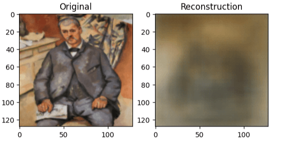
I- that is not ideal. My autoencoder has absolutely butchered this Paul Cezanne artwork - but it clearly demonstrates atleast the compression is working. Plus what do I really expect compressing the image down to a latent space of 1024 dimensions for just 10 epochs? The MSELoss averages out the pixel values, leading to a blurry abstraction as it tries to minimise the loss function. Still, it is pretty cool to see what the model thinks the art looks like deep within its layers.
Where autoencoders truly shine is their ability to abstract and encode abstractions that a normal eye fails to spot. Observing the latent space should give us more insight - is it able to figure out the subtle distinctive quality of each artist?
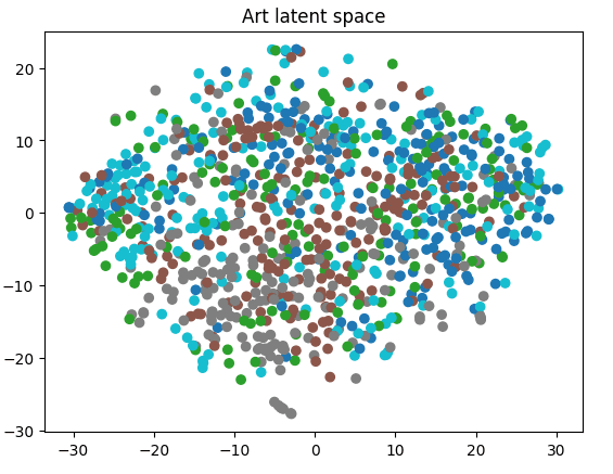
Not quite. There are some micro-clusters if I look really closely, but overall its pretty random. My guess is that it encodes stuff like scenery and color pallete more than the overall aesthetic of each artist.
Learnings
Alas my project seems to have reached a dead end. Autoencoders are quite good at some things, especially anomaly detection. This is not one of those cases. Here, the paintings were too nuanced for the autoencoder to have learned any meaningful difference. There are several ways this might move forward -
- Use a variational autoencoder to see if it does a better job at segmenting the art style.
- Deepen the layers and train for more epochs - 3 layers is hardly deep at all.
- Use a pretrained network like VGG16 to capture semantic similarities of each artwork better.